References

Cell reference is nothing but referring to the position of a cell which is available in the same sheet or different sheet or even different workbook.

In Excel, each row and column has its own name. Each row is identified by its row number and each column is identified by alphabet. In same way, each cell in Excel has its own name. Such as A1, F26 or W345 - consisting of the column letter and row number that intersect at the cell's location. When listing a cell reference, the column letter is always listed first.

One advantage to using cell references in spreadsheet formulas is that, normally, if the data located in the referenced cells changes, the formula or chart automatically updates to reflect the change.

If a workbook has been set not to automatically update when changes are made to a worksheet, a manual update can be carried out by pressing the F9 key on the keyboard.

Formulae	Refer to
=A5	Cell A5
=A1:F4	Cells A1 through F4
=Sheet2!B2	Cell B2 on Sheet2

There are three types of references that can be used in Excel and they are easily identified by the presence or absence of dollar signs ($) within the cell reference.

1.       Relative reference

2.       Absolute reference

3.       Mixed references

Relative Reference

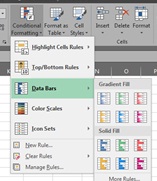
Relative cell references are basic cell references that adjust and change when copied or when using AutoFill. For example, if you copy the formula =A1+B1 from row 1 to row 2, the formula will become =A2+B2. Relative references are especially convenient whenever you need to repeat the same calculation across multiple rows or columns.  By default, all cell references are relative references.

Example:

=SUM(B5:B8), as shown below, changes to =SUM(C5:C8) when copied across to the next cell.

Absolute and Mixed References

There may be times when you do not want a cell reference to change when filling cells. Unlike relative references, absolute references do not change when copied or filled. You can use an absolute reference to keep a row and/or column constant.

                An absolute reference is designated in a formula by the addition of a dollar sign ($).

                It can precede the column reference, the row reference, or both.

Reference	Meaning
$A$2	The column and The row do not change when copied
A$2	The row does not change when copied
$A2	The column does not change when copied

Switch between relative, absolute, and mixed references

1.       Select the cell that contains the formula.

2.       select the reference that you want to change.

3.       Press F4 to switch between the reference types.

Reference

https://www.thoughtco.com/cell-references-relative-absolute-and-mixed-3123401

http://web.pdx.edu/~stipakb/CellRefs.htm

https://support.office.com/en-us/article/Create-or-change-a-cell-reference-c7b8b95d-c594-4488-947e-c835903cebaa

https://www.gcflearnfree.org/excel2016/relative-and-absolute-cell-references/1/

follow us on http://arivilm.blogspot.in/

like us on https://www.facebook.com/Arivilm2501/

Power Pivot (add-in) - an Introduction

PowerPivot is an add-in for Microsoft Excel that enables you to import millions of rows of data from multiple data sources into a single Excel workbook, create relationships between heterogeneous data, create calculated columns and measures using formulas, build PivotTables and PivotCharts, and then further analyze the data so that you can make timely business decisions without requiring IT assistance.

Power Pivot is a feature of Microsoft Excel. It is available as an add-in in Excel 2010 and 2013, and is included natively in Excel 2016. PowerPivot extends a local instance of Microsoft Analysis Services Tabular that is embedded directly into an Excel Workbook. This allows a user to build a ROLAP model in PowerPivot, and use pivot tables to explore the model once it is built. This allows Excel to act as a Self-Service BI platform, implementing professional expression languages to query the model and calculate advanced measures.

Prior to the release of Power Pivot, Microsoft relied heavily on SQL Server Analysis Services as the engine for its Business Intelligence suite. PowerPivot complements the SQL Server core BI components under the vision of one Business Intelligence Semantic Model (BISM), which aims to integrate on-disk multidimensional analytics previously known as Unified Dimensional Model (UDM), with a more flexible, in-memory "tabular" model.

Reference: 

https://msdn.microsoft.com/en-us/library/gg413497(v=sql.110).aspx

https://en.wikipedia.org/wiki/Power_Pivot

follow us on http://arivilm.blogspot.in/

like us on https://www.facebook.com/Arivilm2501/

Conditional Formatting (Session3) - PRESETS

Conditional formatting allows you to automatically apply formatting—such as colors, icons, and data bars—to one or more cells based on the cell value. To do this, you'll need to create a conditional formatting rule.

Conditional Formatting Presets

Excel has several predefined styles—or presets—you can use to quickly apply conditional formatting to your data. They are grouped into three categories:

Data Bars are horizontal bars added to each cell, much like a bar graph.
Color Scales change the color of each cell based on its value. Each color scale uses a two- or three-color gradient. For example, in the Green-Yellow-Red color scale, the highest values are green, the average values are yellow, and the lowest values are red.
Icon Sets add a specific icon to each cell based on its value.

To Use Preset Conditional Formatting:

1.       Select the desired cells for the conditional formatting rule.

2.       Click the Conditional Formatting command. A drop-down menu will appear.

3.       Hover the mouse over the desired preset, then choose a preset style from the menu that appears.

4.       The conditional formatting will be applied to the selected cells.

To remove conditional formatting:

1.       Click the Conditional Formatting command. A drop-down menu will appear.

2.       Hover the mouse over Clear Rules, and choose which rules you want to clear.

3.       The conditional formatting will be removed.

Reference: https://www.gcflearnfree.org/excel2013/conditional-formatting/1/

follow us on http://arivilm.blogspot.in/

like us on https://www.facebook.com/Arivilm2501/

Conditional Formatting (Session2) - Formula-Based Conditional Formatting

Conditional formatting is a fantastic way to quickly visualize data in a spreadsheet. With conditional formatting, you can do things like highlight dates in the next 30 days, flag data entry problems, highlight rows that contain top customers, show duplicates, and more.

Excel ships with a large number of "presets" that make it easy to create new rules without formulas. However, you can also create rules with your own custom formulas. By using your own formula, you take over the condition that triggers a rule, and can apply exactly the logic you need. Formulas give you maximum power and flexibility.

Formula-Based Conditional Formatting

1.       Select the cells you want to format.

2.       Create a conditional formatting rule, and select the Formula option

3.       Enter a formula that returns TRUE or FALSE.

4.       Set formatting options and save the rule.

The ISODD function only returns TRUE for odd numbers, triggering the rule:

Reference : https://exceljet.net/conditional-formatting-with-formulas

follow us on http://arivilm.blogspot.in/

like us on https://www.facebook.com/Arivilm2501/

Conditional Formatting (Session1) - INTRO

Conditional Formatting

Conditional Formatting (CF) is a tool that allows you to apply formats to a cell or range of cells, and have that formatting change depending on the value of the cell or the value of a formula.  When the value of the cell meets the format condition, the format you select is applied to the cell.  If the value of the cell does not meet the format condition, the cell's default formatting is used.

Formatting vs Conditional Formatting

Formatting, such as currency, alignment, and colour, determines how Excel displays a value. But conditional formatting is more flexible, applying specified formatting only when certain conditions are met.

Create conditional formatting rules

                For Example, let say I want to track the student’s marks and their results.

                In this worksheet, we see the information we want by using conditional formatting, driven by two rules that each contain a formula. First rule in the Total column, formats the marks above 300, which is number and second rule is in the Result column formats the result Pass, which is text.

To create the NUMBER rule:

1.       Select cells G2 through G7. Do this by dragging from A2 to A7.

2.       Then, click Home > Conditional Formatting > Highlight Cells Rules > Greater Than.

3.       In the dialog box, enter 300 and select the format you want.

4.       Click OK until the dialog boxes are closed.

5.       The formatting is applied to column G.

6.       In the same way, we can use Lesser Than and Between options. 

To create the TEXT rule:

1.       Select cells G2 through G7. Do this by dragging from A2 to A7.

2.       Then, click Home > Conditional Formatting > Highlight Cells Rules > Text that contains.

3.       In the dialog box, enter Pass and select the format you want.

4.       Click OK until the dialog boxes are closed.

5.       The formatting is applied to column H.

To be continued...

 follow us on http://arivilm.blogspot.in/ 

like us on https://www.facebook.com/Arivilm2501/

People Graph

People Graph is a cool app for Office that transforms your cold data to vivid pictures. The new release includes eight new shapes, simplified data binding, and added new notifications and error handling.

Most people are not aware of the nice tool named People Graph that become available with Excel 2013 and later versions. It is very easy to create a people graph with Excel.  It looks really nice and professional. But it is a one dimensional chart that can only show one column of data.

You can get this app from store link located under Insert Tab.

 Install the People Graph app for Office

1.      Sign in to Office 2013 with your Microsoft Account

2.      Open Excel 2013 and choose INSERT > Apps for Office.

3.      Choose FEATURED APPS, search “People Graph”, and then choose Add.

4.      Choose Trust It.

Chart types

People Graph app includes three chart types.

Chart themes

For each chart type, there are seven themes to choose.

Chart shapes

You can choose from 16 shapes to tell your story.

Here is a step by step guide for creating a People Graph:

1.      Have your data arranged in two columns.

2.      You can find People Graph under insert tab, inside add-ins group.

3.      Click on the button and a default window appears:

Notice two buttons on upper right corner of the screen. The one on the left (looks like a table) is Data button and the one on the right (cog) is Settings button. When you press Data button, a menu will slide in from right.

4.      Input graph title inside the text box below the green button and press “Select your data” button to select your data.

5.      You will receive an information note regarding your selection based on the charts limitations. Press Create button and your People Graph will be created with default styling options.

6.      Now you can change the formatting by Click on the Settings button (Cog on the upper right corner).

follow us on http://arivilm.blogspot.in/

like us on https://www.facebook.com/Arivilm2501/

Slicers

Slicers are visual filters, introduced in Excel 2010. They are a powerful new way to filter pivot table data. Slicers provide buttons that you can click to filter PivotTable data. In addition to quick filtering, slicers also indicate the current filtering state, which makes it easy to understand what exactly is shown in a filtered PivotTable report.

When you select an item, that item is included in the filter and the data for that item will be displayed in the report. For example, when you select East in the Region field, only data that includes East in that field are displayed.

Adding a slicer to a Pivot table

Slicers are typically associated with the PivotTable in which they are created.

1.      Click on any cell in the pivot table 2.      Go to the Insert menu and 3.      Click on Slicer 4.      In the Insert Slicer Box, choose field/s on which you want the slicer. In our case it will be ‘Region’ 5.      Done! Instantly you’ll get an interactive button displaying all four regions. Clicking any region will filter the pivot table

A slicer typically displays the following elements:

1. A slicer header indicates the category of the items in the slicer. 2. A filtering button that is not selected indicates that the item is not included in the filter. 3. A filtering button that is selected indicates that the item is included in the filter. 4. A Clear Filter button removes the filter by selecting all items in the slicer. 5. A scroll bar enables scrolling when there are more items than are currently visible in the slicer. 6. Border moving and resizing controls allow you to change the size and location of the slicer.

Creating interactive charts with slicers

Since slicers talk to Pivot tables, you can use them to create cool interactive charts in Excel. The basic process is like this:

1.      Set up a pivot table that gives you the data for your chart. 2.      Add slicer for interaction on any field (say slicer on customer’s region) 3.      Create a pivot chart (or even regular chart) from the pivot table data. 4.      Move slicer next to the chart and format everything to your taste. 5.      And your interactive chart is ready!

follow us on http://arivilm.blogspot.in/

like us on https://www.facebook.com/Arivilm2501/

Flash fill

Excel’s Flash Fill is a time-saving feature which fills in data for you when a pattern is evident. It can also can extract and insert as well as format and concatenate. This feature can even reverse text, numbers, dates and much more.

ACTIVATE FLASH FILL:

If the Flash Fill does not work automatically, you need to activate in from Excel’s back end by going to:

File > Options > Advanced > Automatically Flash Fill

Separating First Name and Last Name Using Flash Fill

We have a list of full names in one column, and we will separate the data in this column into two individual columns using Flash Fill.

Concatenating Last Name and First Name with Comma Separation

We have a lengthy list of full names in one column, and we wish to have the pattern: last name, comma, first name.

Extracting Initials from Full Names

We have the same list of full names. We will extract initials from the full names using Flash Fill.

Formatting Phone Numbers Using Flash Fill

Using Flash fill to format phone numbers, you can concatenate with brackets to make it easily readable.

Extracting Text before the Symbol @ from Email Addresses

With the Flash fill feature, extracting text before the @ symbol from email addresses is simple.

Note: Flash Fill cannot recognize source data modification. If you apply Flash Fill on source data and then try to modify the source data, Flash Fill cannot recognize the changes and make modifications in available results as Excel formulas do. Therefore, it is best to use Flash Fill with data which is not going to be modified in the future.

follow us on http://arivilm.blogspot.in/

like us on https://www.facebook.com/Arivilm2501/