The Excel TRANSPOSE function
"flips" the orientation of a given range or array. TRANSPOSE converts
a vertical range to a horizontal range, or a horizontal range to a vertical
range. You must enter the TRANSPOSE function as an array formula.
Syntax
The syntax for the TRANSPOSE
function in Microsoft Excel is:
=TRANSPOSE( range )
Parameters or Arguments
range
The range of cells that you
want to transpose.
Transpose Function Examples
Example 1
In the spreadsheet on the
right, the simple vertical range of cells A1-A6 is transposed into the
horizontal range B1-F1.
As shown in the formula bar,
the formula for the function is:
=TRANSPOSE( A1:A6 )
The curly braces { } show that
the function has been input as an Array Formula.
Example 2
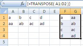
In the spreadsheet on the
right, the range of cells A1-D2 is transposed into the range F1-G4.
In this case, the formula for
the function is:
=TRANSPOSE( A1:D2 )
Again the curly braces { }
shown in the formula bar indicate that the function has been input as an Array
Formula.
Notes
The TRANSPOSE function
converts a vertical range of cells to a horizontal range of cells, or a
horizontal range of cells to a vertical range of cells. Use it to
"flip" a range of cells from one orientation to another.
When array is transposed, the
first row of array is used as the first column of the new array, the second row
of array is used as the second column of the new array, the third row of array
is used as the third column of the new array, and so on.
You must enter the TRANSPOSE
function as an array formula that contains same number of cells as array, using Ctrl+Shift+Enter.
The new array must occupy the
same number of rows as the source array has columns, and the same number of
columns as the source array has rows.
For a one-off conversion, you
can use paste specialt->transpose.
Reference:
follow us on http://arivilm.blogspot.in
like us on https://www.facebook.com/Arivilm2501/


No comments:
Post a Comment